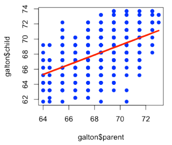
Basic Least Squares
|
1 2 3 4 |
library(UsingR); data(galton) plot(galton$parent,galton$child,pch=19,col="blue") lm1 <- lm(galton$child ~ galton$parent) lines(galton$parent,lm1$fitted,col="red",lwd=3) |
abline() - This function adds one or more straight lines through the current plot.
Inference Basics
|
1 |
sampleLm4$coeff |
|
1 2 |
(Intercept) sampleGalton4$parent 15.8632 0.7698 |
|
1 |
confint(sampleLm4,level=0.95) |
|
1 2 3 |
2.5 % 97.5 % (Intercept) -7.8072 39.534 sampleGalton4$parent 0.4208 1.119 |
A one inch increase in parental height is associated with a 0.77 inch increase in child's height (95% CI: 0.42-1.12 inches).
P-values
|
1 |
confint(lm(galton$child ~ galton$parent),level=0.95) |
|
1 2 3 |
2.5 % 97.5 % (Intercept) 18.4250996 29.4579608 galton$parent 0.5655602 0.7270209 |
|
1 |
summary(lm(galton$child ~ galton$parent))$coeff |
|
1 2 3 |
Estimate Std. Error t value Pr(>|t|) (Intercept) 23.9415 2.81088 8.517 6.537e-17 galton$parent 0.6463 0.04114 15.711 1.733e-49 |
A one inch increase in parental height is associated with a 0.65 inch increase in child's height (95% CI: 0.57-0.73 inches). This difference was statistically significant (P < 0.001).
Speak Your Mind